数值分析课业代写 Problem 1. Program the power method and inverse power method to compute the maximum and minimum eigenvalue/eigenvector pairs of the symmetric
Problem 1.
Program the power method and inverse power method to compute the maximum and minimum eigenvalue/eigenvector pairs of the symmetric matrix A ∈ Rn×n.
To test your code, you can create a random eigenvalue decomposition with specified eigenvalues as follows:
Q = np.random.randn(n, n) # sample a matrix with iid N(0, 1) entries
Q = np.linalg.qr(Q)[0] # the Q factor in its QR decomposition is an
                       # orthogonal matrix sampled uniformly from
                       # the orthgonal group O(n)
Lam = np.diag(...) # set the diagonal matrix of eigenvalues manually
A = Q@Lam@Q.T # compute A from Q and Lam
This way you can fix the values of λ1 and λ2 (or 1/λn and 1/λn−1) to control the convergence rate of the (inverse) power method.
Make a plot (or several plots) of the convergence of the (inverse) power method for several different eigenvalue ratios. Since you set the eigenvalues of your test matrix A yourself, you can easily compare with the true solution. Your plot(s) should show evidence that the convergence rate is largely controlled by, e.g., λ2/λ1.
(Note: in this problem, I would like you to look at both the power method and the inverse power method. For the inverse power method, use np.linalg.lu or scipy.linalg.lu instead of your own LU decomposition to compute the LU decomposition of A. You can then use the function scipy.linalg.solve triangular to do the forward and backward solves involving your triangular factors.)
Incorporate shifts into your power method (i.e., apply the power method and inverse power method to the shifted matrix A − λI). Come up with a strategy for choosing the shift λ to accelerate the convergence of the power method. Note: the shift can vary from iteration to iteration. In general, there can be many possible strategies—you must simply come up with some strategy that reduces the overall number of iterations. However, be careful with the inverse power method: if you change the shift, you must recompute the LU decomposition used to apply (A − λI)−1 at each step.
数值分析课业代写
Read about the compressed sparse row (CSR) sparse matrix format. SciPy provides a class implementing a sparse matrix using the CSR format: see scipy.sparse.csr matrix.
Set up a version of A for N = 64 using scipy.sparse.csr matrix. Next, read the documentation for the function scipy.sparse.linalg.eigsh. Use it to compute the k = 16 smallest nonzero eigenvalues and eigenvectors of A (hint: use the sigma keyword argument).
Using plt.subplot, make a 4 × 4 grid of 2D plots of each of the eigenvectors, as well as a plot of the eigenvalues that you compute.
The matrix A can be interpreted as a graph. Its rows and columns are naturally identified with the nodes in the original lattice, which we think of as the graph’s vertices. There is an edge between a pair of vertices if the corresponding pair of nodes is adjacent in the lattice. Recall from lecture that A is a discretized Laplacian.
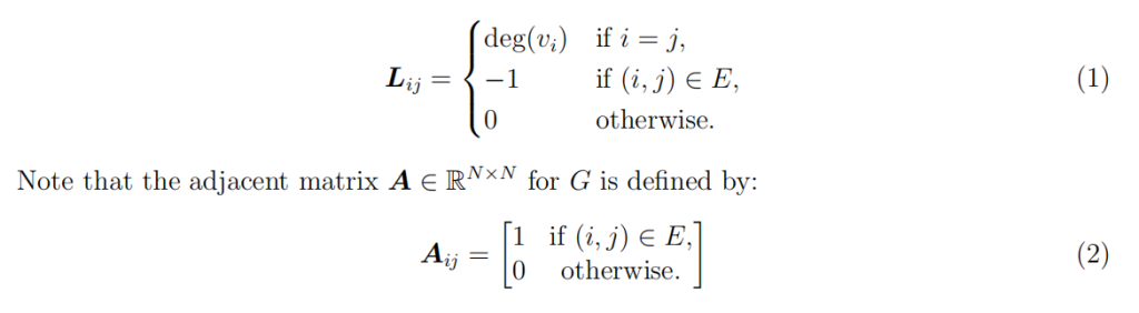
On the other hand, if we start with a graph G = (V, E), where N = |V | and V = {v1, . . . , vN} is the set of vertices and E = {(i, j) : viand vjare adjacent} is the set of edges, we can define the graph Laplacian L ∈ RN×N by:
or some other website online. Load it using Python and build a CSR version of L for your graph. Next, as in Problem 3, use scipy.sparse.linalg.eigsh (note that L should be symmetric!) to compute the first k = 2 smallest nonzero eigenvalue and eigenvector pairs of L. Let u1 and u2 be these eigenvectors, and experiment with making plots of u1 and u2 to visualize the graph. Please be creative and feel free to experiment.
(Hint: the process of getting your graph into Python and building L may be annoying and require some data processing. Don’t be a hero—use a relatively simple graph to make this easy. Between a few hundred vertices and a few thousand vertices is a good target.)
b (bonus).
Compute u3 and make a 3D visualization of your graph. I recommend starting with mplot3d for 3D plotting, but feel free to contact me for more recommendations, and feel free to experiment.
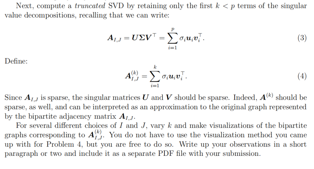
Read about bipartite graphs online. An off-diagonal block of the adjaceny matrix (not the graph Laplacian matrix L!) of your graph from Problem 4 is a bipartite graph. Pick such an off-diagonal block and denote it AI,J, where I and J are the row and column indices of the block (I ∩ J = ∅).
Let m = |I| and n = |J| and p = min(m, n). Compute the singular value decomposition AI,J= UΣV T, where U ∈ Rm×p, V ∈ Rn×p, and Σ ∈ Rp×p. Do this using np.linalg.svd with full matrices=False. Make a semilogy plot of the singular values σ1, . . . , σpand observe how rapidly they decay.
COMP 424 Final Project Game: Colosseum Survival!
AI算法代写 1.Goal The main goal of the project for this course is to give you a chance to play around with some of the AI algorithms discuss...
CSCI 3022 Midterm Exam
数据科学考试代考 Read the following: You may use a calculator provided that it cannot access the internet or store large amounts of data.You may NOT use a
Read the fol...
Volatility Forecasting Homework
波动率预测代写 1.You will estimate the parameters of a few GARCH-type models using about ten years of data (from Jan 1, 2013 to Nov 30, 2022) for SPY
1.
...